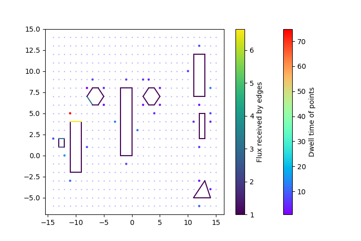
For the Tuesday meeting, I spent some time making heat map visualizations as Prof. Hauser had suggested last week. The idea is that from a visualization of dwell points, it would be useful to not only know which points are dwell-points, but how much time we need to spend at each of them (since some will probably require much more time than others). Another thing that he suggested would be useful is coloring obstacle edges by how much flux each of them receive. We know each of them must receive some minimum flux (as constrained by the linear program) but some edges will definitely receive more than others, and it would be worth it to see how “efficient” our solution is in making all edges get as much flux as required. As a heat map, the variance in coloring over different dwell-times (for the points) and flux-amount (for the obstacle edges) is continuous over some selected color map.

The last weeks have made me realize how great visualizations are. The old adage “a picture is worth a thousand words” certainly carries a weight I’ve disregarded for a long time. When it’s too difficult to parse and crunch numbers directly, a picture can much more easily tell you whether one’s work makes sense or not, and give one an intuition for the sorts of solutions one is getting. For example, last week, Prof. Hauser caught an error in our algorithm by way of a visualization. This week, using the heat map visualizations also lent confidence to the validity of our results. The points we expected to take have large dwell-times did, and the relation between dwell-times and edge flux also made sense.

As discovered last week (to not much surprise), the higher the resolution of a room environment, the longer it takes for our algorithm to run. In fact, it became pretty infeasible to run very high-resolution problems on our computers since it started taking an incredibly large amount of time to complete (and often wouldn’t). Now that we had a functional algorithm, we wanted to build up towards optimizing for speed. To do this, we wanted to figure what was causing this bottle-neck to see if there were any possible fixes. I ran tests, testing each separate module of the algorithm and it turned out that the visibility graph calculation was leeching up time, since the number of potential vantage points increases greatly with increased resolution. In fact, almost all of the run-time was coming from these calculations. I didn’t make any changes to optimize this week, but filed the information away for later.

My mentor was able to get the PRM functionality from Klamp’t to work in the middle of the week, so I started integrating it with the other parts of the code. This was where I ran into OS issues for the second time. Although I installed an Ubuntu subsystem a while back, and it worked for my purposes then, this week I’ve been unable to get the LKH TSP solver to work on Linux, while it works on Window. The trouble is that the executables for Windows and for Linux are different, and in any case, I can’t see beneath the hood to check how they work, so I’m sort of going in blind here. Ultimately, we want our work to function on Linux, so it’ll be necessary to fix that, or find a different solver (unfortunate, because LKH is really great).

This is where we’re lucky, in some sense, because I do in fact have a Windows machine. So, my mentor and I have been exchanging lots of data over the last few days with him sending me PRM results and me feeding them into the LKH solver on Windows to get results. I did spend quite a bit of time on goose chases, trying a different solver (which turned out to be very buggy) and trying to get the LKH solver to work on Linux. Then we found out that my mentor’s PRM code also had a couple errors. It was Friday evening when we were able to figure out the issues and get it to work correctly.

After a few frustrating days, though, it’s great to be able to say that the entire pipeline is complete! At least, it is on Windows. With the PRM distance matrix feeding into the TSP solver, we can finally get a tour through the selected vantage-points and use final path-planners to get the path between pairs of points in the tour. We have an algorithm that, simply given any 2D room with obstacles and a minimum radiation requirement, will find a path through the entire room which irradiates all the surfaces as required!