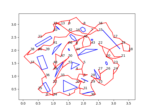
On Monday, I set out to build some test rooms and use the entire pipeline to get disinfection paths through them. I had two main issues; after finding a TSP tour, I was running an optimal path-planner to find the paths between pairs of points set up by that tour. But these optimizing planners were taking far too long to run for very little payoff (because the path length wasn’t that much better than non-optimal paths found by other, faster planners). The more important issue was that the overall paths didn’t look as optimal as one would expect from our entire pipeline. Another way visualizations are incredible! Without them, I wouldn’t have any way of figuring this out. As it is, it was pretty much intuition and looking at the paths to see that they didn’t seem so good:

Looking at this picture, we can see that path is sort of… underwhelming. It goes all over the place instead of taking a nice tour that sort of “circles” all the required points. Something seems wrong here, but since there are so many steps in this pipeline, it’s unclear which one (or ones!) are contributing to the issue. For example, the TSP solver itself is an approximate solver – it doesn’t find the optimal path, so maybe it wasn’t doing a good job. On the other hand, the distances given to the TSP aren’t exact either – they are approximations made by a PRM. Perhaps the wrong distances were causing the solver to work badly. To investigate this, I spent time testing examples on each part of the pipeline separately. On Tuesday, my mentor and I spent a few hours together online trying to figure out what the issue was.

While the video chat was long and quite tiring, we figured out at least one problem; I noticed that in the PRM, one of the settings was preventing two points from connecting in the PRM if they were already in the same connected component.

NOTE: Say we have a set of milestones we want paths between. A probabilistic road-map builds paths by creating a graph where nodes are randomly generated points in free space and edges are created by connecting points which are “directly connectable” in free space. A and B are directly connectable if you can get from point A to point B using the straight line connecting them, which happens if that line doesn’t pass through any obstacles. This PRM continues to grow by randomly generating points atleast until, for each milestone, there is at least one point in the PRM directly connectable to it. This PRM graph can be searched with any graph algorithm to then find a path from one milestone to any other. The way connections are made in the PRM can be controlled (again, because there’s a tradeoff between optimality and runtime, and connecting every single pair of points which can be connected is a huge drain on memory and time). If you prevent your PRM from connecting pairs of points as long as there is some connection between them, your routes will tend to be longer and more winding, because paths between edges that could have been straight-line edges will instead be convoluted, multi-edge paths

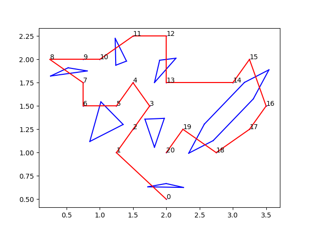
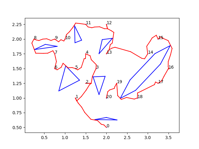
Changing the setting to allow connected component connections made the PRM look a lot better and reduced path lengths. But unfortunately, we were still getting weird overall tours and paths for entire traversals of all the dwell-points. At this point, we were pretty sure it had something to do with the TSP solver. On Thursday, we figured it out; the TSP solver was converting all float values to integer distances by truncating them, meaning that a distance 1 and a distance 1.95 were being taken as the same. The rooms we had tested were all 4 meters x 4 meters, so all dwell-point distances were pretty small. This had been what was screwing up our results. This was fixed by multiplying the adjacency matrix by 10000 (could be any arbitrary large power of 10) so that it took decimal places into account as well. And the new results were … beautiful. Perhaps I’m being biased by the time and effort it took to get here, as well as the unexpected roadblocks, but the results really did look great. Here’s an example tour the TSP solver outputs, followed by the final path we get:

And so, the algorithm was actually finally completed. Now that we have the results, we want to be able to argue why this algorithm is better and more worth using than other existing algorithms for the same problem. Existing solutions to this problem are in actuality pretty sparse; in fact, there’s really only one that’s in practical use currently. So that’s what I’m going to be working on next.